This tutorial will walk you though setting up a simple sequential logic system - namely, a D flip-flop used as a toggle flip-flop. The source of the clock signal will be a Clock block, and the output will be visible with a Scope block (which simulates an oscilloscope display). I'm assuming that you've extracted the library and added it to the Matlab path; if not, go here first. You might also want to walk through the combinational logic tutorial if you haven't done so already.
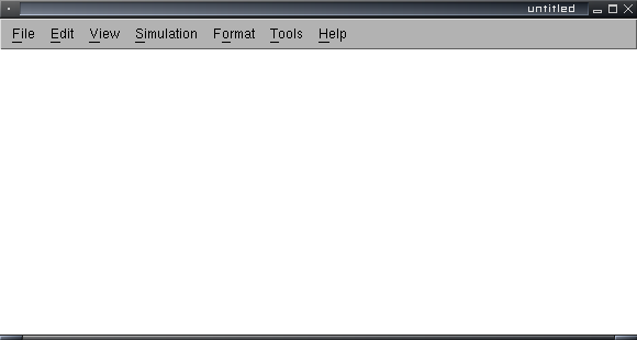
Start up Simulink. Click File, New, Model (or hit Ctrl-N). You should get an empty model window that looks like this:

Go to File, Open, and open up the InputDevs/Sources library. Drag and drop a 'clock' block from the library window you opened earlier into your model. Also drag and drop a 'False' block to your model. Close that library window, go to File, Open (on any library window you have handy; the File menus on all the windows are equivalent), open the Logic directory, and open the 'FlipFlops' library. You should get another library window like this:

Pick the D Flip-Flop that doesn't have the negated clear (it's the one in the middle in the screenshot), and place it in your model. So far, the model should look something like this:

Go back to the main Simulink block library and double-click on the 'Sinks' block library. Drag and drop a 'Scope' into the model; you can close the Sinks after you've got the Scope. In your model, double-click on the Scope block to bring it up. Click the second icon at the top left of the Scope window (the tooltip is 'Parameters'); in the dialog that pops up set the number of axes to 2 instead of 1 and click OK. The scope window should now look like this:

Connect the D input of the flip-flop to the Q' output, the clock block to the CLK input on the flip-flop, the False block to the CLR input, the top input of the scope to the clock, and the bottom input of the scope to the Q output of the flip-flop.
The end result should look like this:

Now go to the Simulation menu and click on 'Configuration Parameters'. Set the Solver options the way I have them in the next screenshot:

The two changes are Type to 'Fixed-step' and Solver to 'discrete'.
Now you can let it rip! Click Simulation, Start. If all goes well, two traces should appear in the Scope window and then the simulation should terminate. This is because the simulation was set to run from time=0 to time=10 (the units are arbitrary) with an unconstrained sample time. If you want it to run in close to real time and not stop automatically, set the simulation's end time to 'inf' and the fixed-step size to '1e-4'; this makes the time scale work out to more or less 1 time unit per second on modern machines. There doesn't seem to be a way to make the simulaton run in a real-time mode with 1 time unit being exactly 1 second.
Screenshot of what should have happened on the Scope:

Some blocks (such as the Clock block) have a configuration dialog that opens when you double-click them; on the Clock you can use it to set the period and duty cycle (ratio of on time to off time).
You can download the completed example here.